rand_binomial

rand_binomial(size, prob, netrep='graphlet', nettype='bu', initialize='zero', netinfo=None, randomseed=None)

Creates a random binary network following a binomial distribution.

Parameters:

• size (list or array of length 2 or 3.) – Input [n,t] generates n number of nodes and t number of time points. Can also be of length 3 (node x node x time) but number of nodes in 3-tuple must be identical.
• prob (int or list/array of length 2.) –

  If int, this indicates probabability for each node becoming active (equal for all nodes).

  If tuple/list of length 2, this indicates different probabilities for edges to become active/inactive.

  The first value is “birth rate”. The probability of an absent connection becoming present.

  The second value is the “death rate”. This dictates the probability of an active edge remaining present.

  example : [40,60] means there is a 40% chance that a 0 will become a 1 and a 60% chance that a 1 stays a 1.

• netrep (str) – network representation: ‘graphlet’ (default) or ‘contact’.
• nettype (str) – Weighted or directed network. String ‘bu’ or ‘bd’ (accepts ‘u’ and ‘d’ as well as b is implicit)
• initialize (float or str) – Input percentage (in decimal) for how many nodes start activated. Alternative specify ‘zero’ (default) for all nodes to start deactivated.
• netinfo (dict) – Dictionary for contact representaiton information.
• randomseed (int) – Set random seed.

Returns:

net – Generated nework. Format depends on netrep input argument.

Return type:

array or dict

Notes

The idea of this function is to randomly determine if an edge is present.

Option 2 of the “prob” parameter can be used to create a small autocorrelaiton or make sure that, once an edge has been present, it never disapears. [rb-1]

Examples

>>> import teneto
>>> import numpy as np
>>> import matplotlib.pyplot as plt

To make the networks a little more complex, the probabailities of rand_binomial can be set so differently for edges that have previously been active. Instead of passing a single integer to p, you can pass a list of 2 values. The first value is the probabililty for edges that, at t-1=0 will be active at t (is sometimes called the birth-rate). The second (optional) value is the probabaility of edges that, at t-1=1 will be active at t (sometimes called the death-rate). The latter value helps create an autocorrelation. Without it, connections will have no autocorrelation.

Example with just birthrate

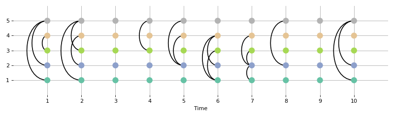
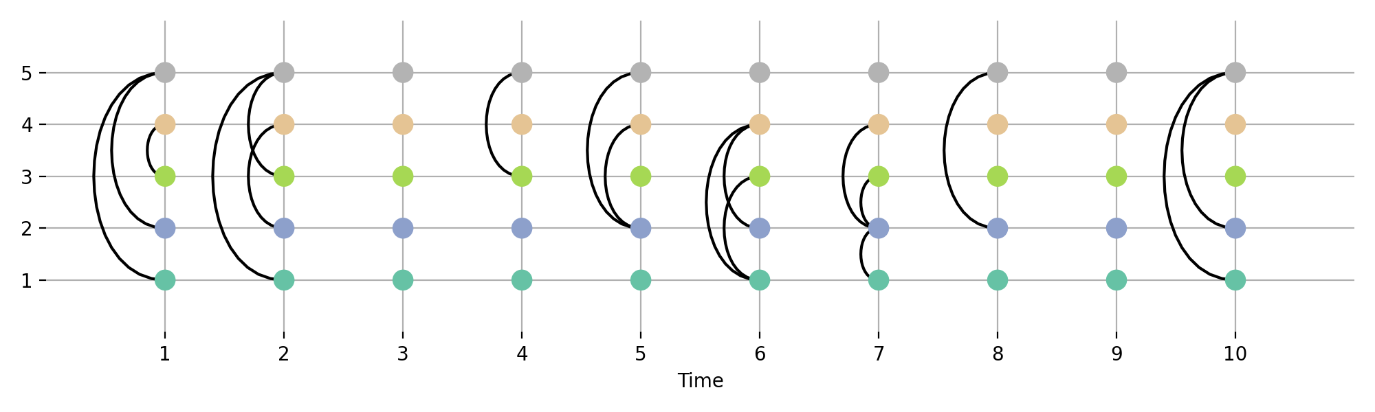
Below we create a network with 5 nodes and 10 time-points. Edges have a 25% chance to appear.

>>> np.random.seed(2017) # For reproduceability
>>> N = 5 # Number of nodes
>>> T = 10 # Number of timepoints
>>> birth_rate = 0.25
>>> G = teneto.generatenetwork.rand_binomial([N,N,T], [birth_rate])

We can see that that edges appear randomly:

>>> fig,ax = plt.subplots(figsize=(10,3))
>>> ax = teneto.plot.slice_plot(G, ax, cmap='Set2')
>>> fig.tight_layout()
>>> fig.show()

(Source code, png, hires.png, pdf)

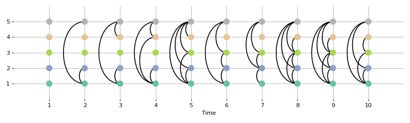
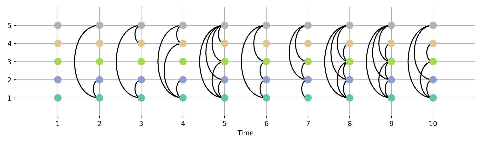
Example with birthrate and deathrate

Below we create a network with 5 nodes and 10 time-points. Edges have a 25% chance to appear and have a 75% chance to remain.

>>> np.random.seed(2017) # For reproduceability
>>> N = 5 # Number of nodes
>>> T = 10 # Number of timepoints
>>> birth_rate = 0.25
>>> death_rate = 0.75
>>> G = teneto.generatenetwork.rand_binomial([N,N,T], [birth_rate, death_rate])

We can see the autocorrelation that this creates by plotting the network:

>>> fig,ax = plt.subplots(figsize=(10,3))
>>> ax = teneto.plot.slice_plot(G, ax, cmap='Set2')
>>> fig.tight_layout()
>>> fig.show()

(Source code, png, hires.png, pdf)

References

[rb-1]

Clementi et al (2008) Flooding Time in edge-Markovian Dynamic Graphs PODC This function was written without reference to this paper. But this paper discusses a lot of properties of these types of graphs.