What are temporal networks?¶

Temporal networks are, quite simply, network representations that flow through time. They are useful for analysing how a connected system develops, changes or evolves through time. This change in time can depict how information spreads along with a social network or how different brain areas cooperate to perform a task.

This page introduces some of the basic concepts of temporal network theory.

Node and edges: the basics of a network¶

A network is a representation of something using a graph from mathematics. This something can be a representation of an empirical phenomenon or a simulation. A graph contains nodes (sometimes called vertices) and edges (sometimes called links).

Nodes and edges can represent a vast amount of different things in the world. For example, nodes can be friends, cities, or brain regions. Edges between could represent trust relationships, train lines, and neuronal communication.

The flexibility in what nodes are is one of the reasons network theory is very interdisciplinary. The benefits of having network representation are that similar analysis methods can be applied, regardless of what the underlying node or edge represents. This abstractness means that network theory is a very inter-disciplinary subject. However, it also entails that certain concepts have multiple names (e.g. nodes and vertices).

With a network, you can analyse for example, if there is any “hub” node. In transportation networks, there are often hubs which connect many different areas where passengers usually have to change at (e.g. airports like Frankfurt, Heathrow or Denver). In social networks, you can quantify how many steps it is to another person in that network (see the famous six steps to Kevin Bacon).

Mathematically, A network if often referenced as G or \(\mathcal(G)\); i and j are indices of nodes; a tuple (i,j) reference an edge between nodes i and j. G is often expressed in the form of a connectivity matrix (or adjacency matrix) \(A_{ij} = 1\) if a connection is present and \(A_{ij} = 0\) if a connection is not present. The number of nodes if often referenced to as N. Thus, A is a N x N matrix.

Different network types¶

There are a few different versions of networks. Two key distinctions are:

Are the connections binary or weighted.
Are the connections undirected or directed.

If a connection is binary, then (as in the section above) an edge is either present or not. When adding a weight-value, an edge becomes a 3-tuple (i,j,w) where w is the magnitude of the weight. And in the connectivity matrix, \(A_{ij} = w\). Often the weight is between 0 and 1 or -1 and 1, but this does not have to be the case.

When connections are undirected, it means that both nodes share the connection. Examples of such networks can be if two cities are connected by train lines. For such networks \(A_{ij} = A_{ji}\). With directed edges, it means that the connection goes from i to j. Examples of these types of networks can be citation networks. If a scientific article i cites another article j, it is not common for j to also cite i. So in such cases, \(A_{ij}\) does not need to equal \(A_{ji}\). It is the common notation for the source node (sending the information) to be first and the target node (receiving the information) to be second.

Adding a time dimension¶

In the above formulation of networks \(A_{ij}\) only has one edge. In a temporal network, a time-stamp is also included in the edge’s tuple. Thus, binary edges are now expressed as 3-tuples (i,j,t) and weighted networks as 4 tuples (i,j,t,w). Connectivity matrices are now three dimensional: \(A_{ijt} = 1\) in binary and \(A_{ijt} = w\) in weighted networks.

The time indices are an ordered sequence. This ordering can now reveal information about what is occurring in the network through time.

For example, using friends’ lists from social network profiles can be used to create a static network about who is friends with who. However, imagine one person enters a group of friends, by seeing when everyone become friends, this gives the network more explanatory power.

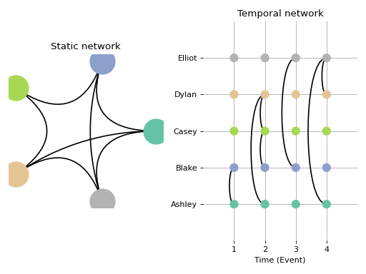
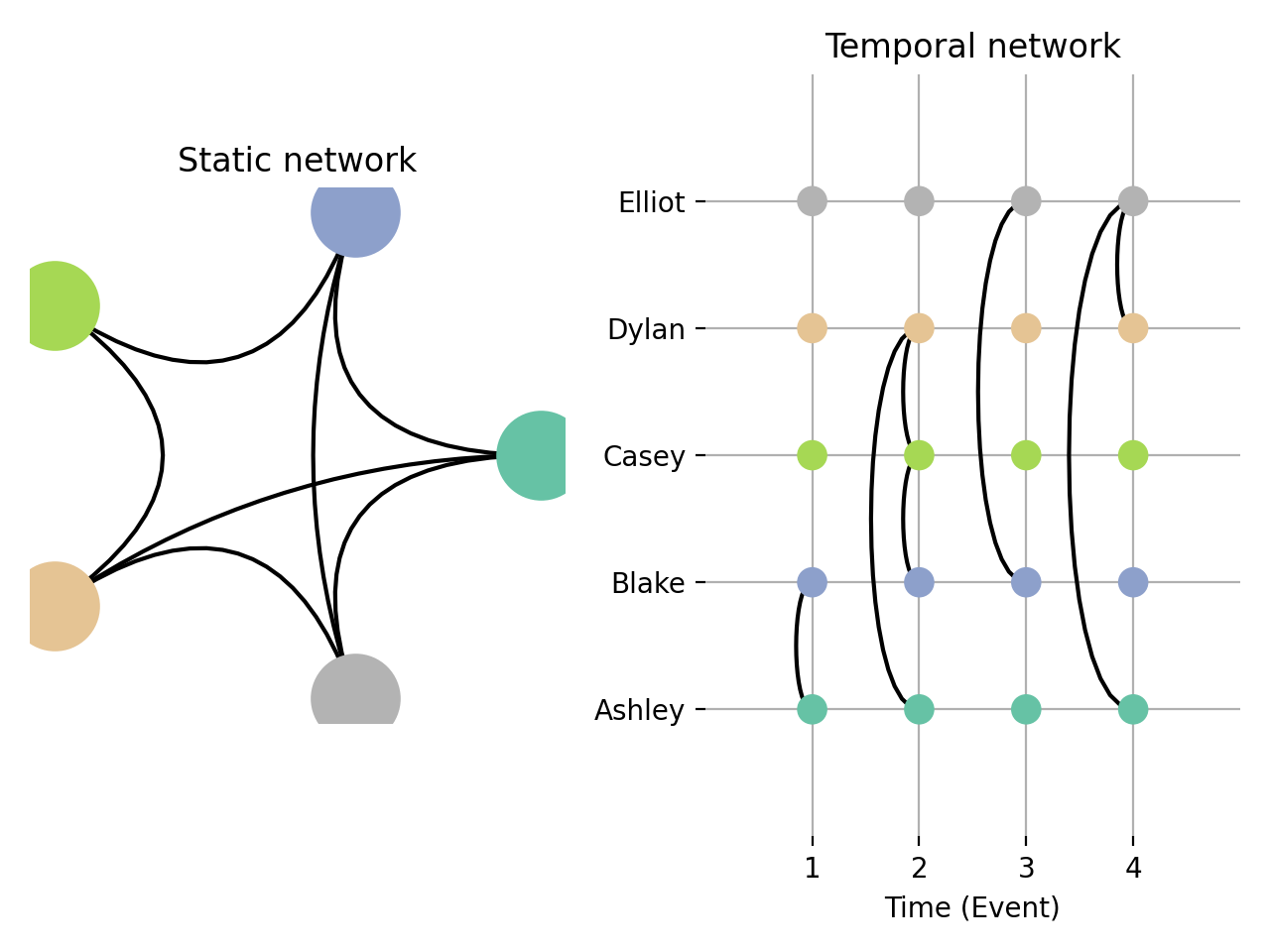
Compare the following two figures representing meetings between friends:

(Source code, png, hires.png, pdf)

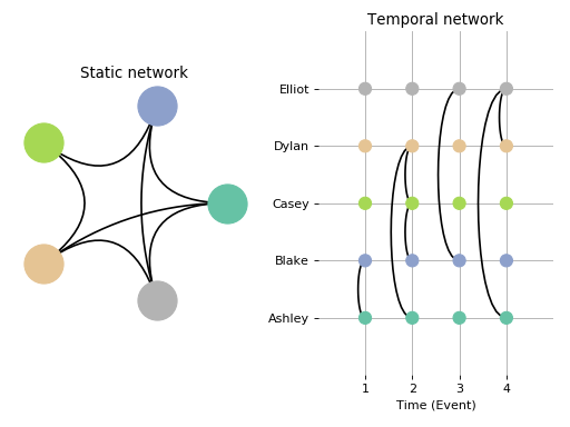
In the static network, on the left, each person (node) is a circle, and each black line connecting the rings is an edge. In this figure, we can see that everyone has met everyone except Dylan (orange) and Casey (light green).

The slice_plot on the left shows nodes (circles) at multiple “slices” (time-points). Each column represents of nodes represents one time-point. The black line connecting two nodes at a time-point signifies that they met at that time-point.

In the temporal network, we can see a progression of who met who and when. At event 1, Ashley and Blake met. Then A-D all met together at event 2. At event 3, Blake met Dylan. And at event 4, Elliot met Dylan and Ashley (but those two themselves did not attend). This depiction allows for new properties to be quantified that missed in a static network.

What is time-varying connectivity?¶

Another concept that is often used within fields such as cognitive neuroscience is time-varying connectivity. Time-varying connectivity is a larger domain of methods that analyse distributed patterns over time where temporal network theory is one set of analysis methods within it. Temporal network theory analyses time-varying connectivity representations that consist of time-stamped edges between nodes. There are other alternatives to analyse such representations and other time-varying connectivity representations as well (e.g. temporal ICA).

What is teneto?¶

Teneto is a python package that can several quantify temporal network measures (more are being added). It can also use methods from time-varying connectivity to derive connectivity estimate from time-series data.